The Hidden Math Behind Machine Learning – AI Principles
Introduction: Demystifying Machine Learning: The Essential Mathematical Foundations for Technologists
Machine learning principles have transformed how software applications function in today’s digital landscape. Between 2017 and 2018, McKinsey research found the percentage of companies embedding at least one AI capability in their business processes more than doubled, with nearly all companies using AI reporting some level of value. This rapid adoption highlights why understanding the fundamentals behind these systems has become increasingly important.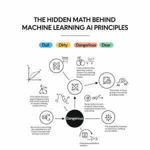
Essentially, machine learning helps software applications become more accurate at predicting outcomes without being explicitly programmed. The primary goal of machine learning is to enable systems to learn from data, identify patterns, and make decisions with minimal human intervention. Businesses across industries use these capabilities to improve efficiencies, perform preventative maintenance, adapt to market conditions, and leverage consumer data.
The 8 principles of responsible machine learning development provide a practical framework for technologists when designing, developing, and maintaining systems that learn from data. However, behind these principles lies a foundation of mathematical concepts that many find intimidating. This article demystifies the hidden mathematics that powers machine learning algorithms, explaining complex ideas in straightforward terms without sacrificing accuracy.
By understanding the mathematical foundations—from data representation and optimization to probability and linear algebra—readers will gain deeper insights into how machine learning systems actually work. Whether you’re a business leader evaluating AI solutions or a developer beginning your machine learning journey, grasping these fundamentals will help you make more informed decisions about implementing and using these powerful technologies.
Table of Contents
The Role of Math in Machine Learning Foundations
“”Mathematics is the science of patterns, and nature exploits just about every pattern that there is.”” — Ian Stewart, Emeritus Professor of Mathematics, University of Warwick; renowned popular mathematics author
Mathematics serves as the backbone of machine learning algorithms, providing the theoretical framework that makes intelligent systems possible. Unlike traditional programming where rules are explicitly coded, machine learning relies on mathematical models that evolve through exposure to data. Statistics and [mathematical optimization](https://en.wikipedia.org/wiki/Machine_learning) comprise the foundations of machine learning, enabling computers to recognize patterns and make decisions with increasing accuracy over time.
Why math is essential in ML algorithms
Mathematics is not merely a tool but the very foundation upon which machine learning stands. Without a strong mathematical understanding, developing effective machine learning solutions becomes nearly impossible for several reasons:
First, mathematical concepts allow engineers to select appropriate algorithms and parameters. From choosing efficient training times to managing complexity and bias-variance trade-offs, mathematical knowledge guides every decision in the machine learning process.
Second, mathematics provides the analytical framework needed to understand how algorithms function. For instance, calculus—particularly differential calculus—enables the optimization of model parameters through techniques like gradient descent. Similarly, linear algebra supports critical operations in neural networks through matrix multiplication.
The core mathematical disciplines essential for machine learning include:
- Linear Algebra: Crucial for representing and manipulating data through vectors, matrices, eigenvalues, and vector spaces
- Calculus: Fundamental for optimization techniques, especially in gradient descent and backpropagation
- Probability and Statistics: Essential for making inferences, understanding uncertainty, and building probabilistic models
- Optimization Theory: Necessary for minimizing or maximizing objective functions to improve model performance
Fundamentally, machine learning algorithms learn through mathematical processes rather than explicit programming. Understanding statistical distributions helps in feature engineering and dataset evaluation, while probability theory enables proper risk assessment and uncertainty quantification.
What is the primary goal of machine learning?
The primary goal of machine learning is to enable systems to learn from data, identify patterns, and make decisions with minimal human intervention. Tom M. Mitchell provided a widely quoted definition: “A computer program is said to learn from experience E with respect to some class of tasks T and performance measure P if its performance at tasks in T, as measured by P, improves with experience E“. This definition emphasizes the operational aspect of machine learning rather than defining it in cognitive terms.
Modern machine learning has two principal objectives. The first is to classify data based on developed models. The second is to make predictions for future outcomes using these models. These objectives align with the fundamental purpose of training machines to improve at tasks without explicit programming.
Additionally, machine learning aims to extract meaningful patterns from data that can lead to actionable insights. Whether applied to web search ranking, financial risk evaluation, customer churn prediction, or autonomous vehicles, the underlying goal remains consistent: to create systems that continuously improve through exposure to more data.
To achieve these objectives, several steps must occur: data collection and preparation, algorithm selection, model evaluation, hyperparameter tuning, and finally making predictions. Throughout this process, mathematics provides the language and tools needed to transform raw data into valuable insights and accurate predictions.
Principle 1: Data Representation and Vector Spaces
Data representation forms the foundation upon which machine learning algorithms operate and learn. At its core, machine learning depends on converting real-world information into mathematical structures that computers can process. This transformation enables algorithms to detect patterns, make predictions, and generate insights that would otherwise remain hidden in complex datasets.
Feature vectors and dimensionality
Machine learning models ingest data through floating-point arrays called feature vectors, which serve as numerical representations of objects or phenomena. These vectors contain multiple elements that collectively describe the properties of what they represent. For instance, an image might be represented by pixel values, while text documents could be encoded using word frequencies.
Feature vectors occupy what mathematicians call a “feature space” – a mathematical construct where each dimension corresponds to a specific feature or attribute. Consequently, a dataset with ten features creates a ten-dimensional space where each data point exists as a specific coordinate. This vector space representation enables mathematical operations essential for machine learning algorithms to function properly.
Feature engineering, the process of converting raw data into suitable representations for models, stands as a crucial step in machine learning workflows. During this process, practitioners transform raw dataset values into more effective representations through techniques like:
- Normalization (scaling values to similar ranges)
- Binning (grouping continuous values into discrete categories)
- One-hot encoding (converting categorical data into numerical format)
Furthermore, the structure of feature vectors varies based on the application domain. In computer vision applications, features might represent gradient magnitude, color values, or edges. For speech recognition, vectors might encode sound lengths or noise ratios, whereas spam detection might utilize features like IP location or word frequency patterns.
As the number of dimensions in a feature space increases, a phenomenon known as the “curse of dimensionality” emerges. This occurs because as dimensionality grows, the volume of the space expands exponentially, causing data to become increasingly sparse. For algorithms that rely on distance measurements, this sparsity creates significant challenges, as most high-dimensional space remains empty.
Euclidean distance in KNN and clustering
Euclidean distance serves as the most widely used distance measure in machine learning, calculating the straight-line distance between two points in n-dimensional space. For two points p and q in n-dimensional space, the Euclidean distance formula is:
d(p,q) = √Σ(pᵢ – qᵢ)²
This measurement forms the mathematical backbone of numerous machine learning algorithms, notably K-Nearest Neighbors (KNN) and clustering techniques. In KNN, a supervised learning classifier, the algorithm classifies data points based on the class labels of their k-nearest neighbors. The proximity between points, typically measured using Euclidean distance, determines which neighbors influence the classification decision.
Besides Euclidean distance, other distance metrics exist, including:
- Manhattan distance (L1 norm): Measures the absolute sum of differences between coordinates, representing movement along grid lines
- Minkowski distance: A generalized form where p=1 yields Manhattan distance and p=2 produces Euclidean distance
- Hamming distance: Used primarily with boolean vectors to count positions where vectors differ
The choice of distance measure significantly impacts clustering results, influencing the shape and structure of the clusters formed. Although Euclidean distance remains the default in many algorithms, its effectiveness diminishes in high-dimensional spaces. As dimensionality increases, the difference in distances between data points becomes negligible, making it difficult for algorithms to distinguish between similar and dissimilar points.
Vector space models enable similarity comparisons between objects by calculating distances or angles between their vector representations. For text documents, cosine similarity often provides better results than Euclidean distance, as it measures the angle between vectors rather than their absolute distance. This approach proves particularly useful when the magnitude of vectors is less important than their directional relationship.
Through proper data representation and thoughtful selection of distance metrics, machine learning algorithms gain the ability to quantify similarities, detect patterns, and make accurate predictions based on mathematical relationships in the feature space.
Principle 2: Optimization and Cost Functions
Optimization lies at the heart of training effective machine learning models, serving as the mathematical mechanism through which algorithms learn from data. Through carefully designed cost functions and optimization techniques, models iteratively improve their performance until reaching optimal or near-optimal solutions.
Gradient descent and loss minimization
Loss functions quantify the discrepancy between predicted and actual values, providing a single numerical metric that measures model performance. Primarily, loss functions guide the optimization process by offering feedback that helps algorithms adjust their parameters. Common loss functions include:
- Mean Squared Error (MSE): Calculates the average squared difference between predictions and expected results, penalizing larger errors more heavily
- Mean Absolute Error (MAE): Computes the average of absolute differences, less sensitive to outliers than MSE
- Huber Loss: Combines advantages of MSE and MAE, less sensitive to outliers while maintaining differentiability
- Cross-Entropy Loss: Used for classification tasks, ensures even small probability errors are penalized
Gradient descent subsequently minimizes these loss functions by iteratively adjusting model parameters. The algorithm works by calculating the gradient (slope) of the loss function with respect to each parameter, then moving in the opposite direction of the gradient. This process repeats until the model converges—when further iterations no longer significantly reduce the loss.
The learning rate, a critical hyperparameter, determines the step size during optimization. Too small a learning rate results in slow convergence, whereas too large a rate may cause overshooting and divergence.
Convex vs non-convex functions in ML
The optimization landscape in machine learning typically involves either convex or non-convex functions, which dramatically affects the ease of finding optimal solutions.
Convex functions possess a key advantage: any local minimum is also the global minimum. This property enables gradient descent to reliably converge to the optimal solution given appropriate learning rates. Linear regression models, indeed, always produce convex loss surfaces.
Non-convex functions, conversely, contain multiple local minima, making global optimization more challenging. Most deep learning models use non-convex loss functions due to their complex architectures. For these scenarios, algorithms like Stochastic Gradient Descent (SGD) perform better by introducing randomness that helps escape local minima.
Despite these challenges, optimization algorithms continue to evolve, with variants like Momentum, RMSProp, and Adam improving convergence rates for both convex and non-convex problems.
Principle 3: Probability and Statistical Inference
“”One of the pleasures of looking at the world through mathematical eyes is that you can see certain patterns that would otherwise be hidden.”” — Steven Strogatz, Jacob Gould Schurman Professor of Applied Mathematics, Cornell University; leading expert in applied mathematics and network theory
Probability theory underpins the decision-making capabilities of machine learning algorithms, enabling systems to handle uncertainty and make predictions based on incomplete information. As machine learning models must often operate in environments where certainty is impossible, statistical inference provides the mathematical framework necessary for working with probabilities rather than absolutes.
Bayes’ Theorem in Naive Bayes classifiers
Bayes’ Theorem offers a principled approach to calculating conditional probabilities, effectively “inverting” the conditions to find P(X|Y) from P(Y|X). Mathematically expressed as:
P(X|Y) = [P(Y|X) × P(X)] / P(Y)
Where:
- P(X|Y) is the posterior probability
- P(Y|X) is the likelihood
- P(X) is the prior probability
- P(Y) is the marginal likelihood or evidence
This theorem forms the foundation for Naive Bayes classifiers, a family of probabilistic algorithms widely used in text classification and spam filtering. The “naive” aspect refers to the assumption that all features are conditionally independent given the class. Hence, Naive Bayes simplifies the joint probability model to:
P(Ck|x) ∝ P(Ck) × ∏ P(xi|Ck)
Accordingly, the classifier assigns the class label that maximizes this posterior probability. The conditional independence assumption, though rarely true in real-world scenarios, makes computation tractable. Even with this simplification, Naive Bayes classifiers perform remarkably well, requiring minimal training data.
Maximum likelihood estimation (MLE)
Maximum likelihood estimation represents a fundamental statistical approach for parameter estimation in machine learning models. MLE works by finding parameter values that maximize the likelihood function—making the observed data most probable under the assumed model.
For a dataset X = {x₁, x₂, …, xₙ}, MLE finds parameters θ that maximize:
L(θ|X) = P(X|θ)
In practice, to avoid numerical issues with multiplying small probabilities, the log-likelihood is often used instead:
log L(θ|X) = ∑ log P(xi|θ)
MLE serves as the mathematical backbone for many machine learning algorithms, including logistic regression, Gaussian Mixture Models, and Hidden Markov Models. Furthermore, from a Bayesian perspective, MLE equates to maximum a posteriori estimation with uniform prior distributions.
Among MLE’s key properties: as sample size increases, estimates become consistent (converging to true values), efficient (achieving the Cramér–Rao lower bound), and asymptotically normal. Through this approach, models can systematically learn from data, adapting their parameters to best explain observed patterns.
Principle 4: Linear Algebra and Matrix Operations
Linear algebra provides the mathematical machinery that powers many machine learning algorithms, serving as the computational foundation for everything from basic data analysis to complex deep learning models. Through matrix operations, algorithms manipulate high-dimensional data efficiently, enabling complex transformations that would otherwise be computationally prohibitive.
Matrix multiplication in neural networks
Neural networks fundamentally rely on matrix multiplication to process information through their layers. At their core, the execution of neural networks involves linear algebra structures multiplied and added together. During forward propagation, inputs from one layer multiply with weights to produce outputs for the next layer, making matrix multiplication the primary computational operation.
For example, in a simple neural network layer, if matrix A represents weights of size m×n and matrix B represents inputs of size n×p, their product C will be of size m×p. This operation computes weighted sums for each neuron in a single mathematical step:
C = A·B where Cᵢⱼ = Σ(Aᵢₖ × Bₖⱼ)
The efficiency of matrix operations explains why modern frameworks like Google’s TensorFlow incorporate “tensor” in their name—tensors being matrices with more than two dimensions. In practice, these operations allow networks to process entire batches of inputs simultaneously, vastly improving computational efficiency.
GEMMs (General Matrix Multiplications), defined as C = αAB + βC, form the fundamental building blocks for many neural network operations. These include fully-connected layers, recurrent layers, and even convolutional layers after appropriate transformations.
Eigenvalues in PCA for dimensionality reduction
Principal Component Analysis (PCA) represents one of the most powerful applications of linear algebra in machine learning, using eigenvalues and eigenvectors to reduce data dimensionality while preserving information.
PCA transforms original datasets into a new coordinate system structured by principal components. These components, which are the eigenvectors of the data’s covariance matrix, represent directions of maximum variance in the data. The corresponding eigenvalues indicate how much variance each component captures.
Mathematically, eigenvectors and eigenvalues emerge from solving the characteristic equation:
det(A - λI) = 0
Where A is the covariance matrix, λ represents eigenvalues, and I is the identity matrix.
The significance of eigenvalues becomes apparent in dimensionality reduction—larger eigenvalues correspond to directions containing more information. By ranking eigenvectors by their eigenvalues and selecting only those with the highest values, PCA effectively compresses data while minimizing information loss.
For instance, in a dataset with 50 variables, if only four eigenvalues are significantly large (e.g., 50, 29, 17, 10, followed by much smaller values like 2, 1, 0.4…), the dimensionality can be reduced from 50 to just 4 dimensions. This reduction simplifies visualization and prevents overfitting in machine learning models.
Conclusion
Mathematics serves as the fundamental backbone that enables machine learning systems to function effectively. Throughout this article, we explored four essential mathematical principles that power modern machine learning algorithms. Data representation through vector spaces allows computers to process real-world information mathematically, while distance metrics help quantify similarities between data points. Subsequently, optimization techniques like gradient descent enable models to learn from their mistakes, continuously refining parameters to minimize error.
Additionally, probability theory equips machine learning systems to handle uncertainty and make predictions based on incomplete information. Concepts like Bayes’ Theorem and maximum likelihood estimation provide the statistical framework necessary for algorithms to learn from observed data. Finally, linear algebra operations form the computational foundation that makes complex transformations possible, especially within neural networks where matrix multiplication drives information processing.
Understanding these mathematical principles offers several advantages. First, it helps practitioners select appropriate algorithms and parameters for specific problems. Second, this knowledge enables more efficient troubleshooting when models underperform. Third, it provides insight into the limitations and capabilities of different machine learning approaches.
The significance of these mathematical foundations extends beyond technical implementation. As machine learning continues to transform industries from healthcare to finance, those who grasp these underlying principles will be better positioned to develop responsible and effective AI systems. Though the mathematics may initially seem daunting, the concepts presented here demonstrate that these foundations can be understood without advanced mathematical training.
Ultimately, machine learning represents the practical application of mathematical principles to solve complex problems. The algorithms do not possess true intelligence but rather apply statistical patterns and optimization techniques to data. This mathematical foundation explains both the remarkable capabilities and current limitations of machine learning systems. Armed with this understanding, practitioners can build more robust models while business leaders can make more informed decisions about implementing these powerful technologies.
Key Takeaways
Understanding the mathematical foundations behind machine learning empowers better decision-making in AI implementation and reveals how these powerful systems actually function beneath the surface.
• Math is the backbone of ML: Linear algebra, calculus, probability, and optimization theory provide the essential framework that enables algorithms to learn patterns and make predictions from data.
• Data becomes vectors for processing: Machine learning transforms real-world information into mathematical feature vectors in high-dimensional spaces, enabling algorithms to quantify similarities and detect patterns.
• Optimization drives learning: Gradient descent and cost functions allow models to iteratively improve by minimizing prediction errors, with the learning process being fundamentally mathematical rather than cognitive.
• Probability handles uncertainty: Bayes’ Theorem and statistical inference enable ML systems to make decisions with incomplete information, forming the basis for classification and prediction algorithms.
• Matrix operations power neural networks: Linear algebra, particularly matrix multiplication and eigenvalue decomposition, provides the computational foundation for complex transformations in deep learning and dimensionality reduction.
These mathematical principles explain both the remarkable capabilities and current limitations of machine learning systems, helping practitioners build more robust models while enabling business leaders to make informed AI implementation decisions.
FAQs
Q1. What are the key mathematical foundations of machine learning? The essential mathematical foundations of machine learning include linear algebra, calculus, probability and statistics, and optimization theory. These disciplines provide the framework for data representation, algorithm optimization, statistical inference, and complex computations in neural networks.
Q2. How does machine learning work in simple terms? Machine learning enables computers to learn from data and make decisions or predictions without explicit programming. It involves creating algorithms that can identify patterns in data, improve their performance through experience, and make data-driven decisions with minimal human intervention.
Q3. Why is mathematics crucial for understanding machine learning? Mathematics is crucial because it forms the backbone of machine learning algorithms. It allows for proper data representation, enables the selection of appropriate algorithms and parameters, provides the analytical framework to understand how algorithms function, and is essential for optimizing model performance and interpreting results.
Q4. What are the three main components of a machine learning model? The three main components of a machine learning model are representation (how the data is structured and presented to the algorithm), evaluation (how the model’s performance is measured), and optimization (how the model improves its performance over time).
Q5. How is linear algebra used in neural networks? Linear algebra is fundamental in neural networks, particularly through matrix operations. Matrix multiplication is used to process information through network layers, enabling efficient computation of weighted sums for each neuron. This allows neural networks to handle complex transformations and process large amounts of data simultaneously.